Confidence Intervals

This post discusses about confidence intervals used in statistics. Look at the questions listed and then read through the notes to understand better!

---

Questions to ask:

1. What are the 2 parts of Inferential statistics?
2. What is Estimation? what are its types?
3. What is point estimation? What are the most common point estimators?
4. What is Sampling Distribution? Is it plotted in real life?
5. What happens when you increase the sample size?
6. What are confidence intervals/interval estimation?
7. What is Standard error? How is it related to confidence interval?
8. What is the central limit theorem?
9. What does 95% confidence interval mean?

---

Statistical Inference can be broken into 2 parts:

1. Estimation
   1. Point Estimation
   2. Interval Estimation (confidence intervals)
2. Hypothesis testing

Estimation

In Estimation, we are concerned with ‘estimating’ the values of specific population parameters. For example, to find the mean weight of adults of a country, we create a sample to ‘estimate’ the mean. The sample mean is the point estimate of the true population mean is that sample mean.

The 2 major point estimates measured are

• Mean
• Proportion (percentage of True/desired)

Sampling Distribution of an Estimator

Let us assume the task is to find the mean weight of 1000 adults in an office.

• We take a random sample of 50 people
• Obtain a sample mean, and plot it in histogram
• repeat this n times

This leads us to a histogram, where the weight might be distributed from 45 to 95 kgs, with a lot of samples nearing 70Kgs, and decreases either side. This is the sampling distribution.

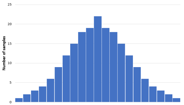
This is a conceptual model, as in practice, we do not get chances to resample and rework our calculations.

Increasing the sample size causes 2 effects:

1. The reduction in the standard error -> reduces the variance in the distribution
2. The distribution/histogram becomes symmetrical and looks like a normal distribution. -> Central limit theorem.

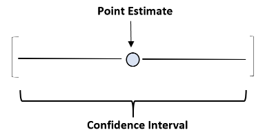
Although a point estimate represents our best possible estimate of some true population parameter, it’s unlikely that it will exactly match the population parameter. So, to capture this uncertainty we can create a confidence interval – a range of values that is likely to contain a population parameter with a certain level of confidence

We refer to the amount of variability in terms of the uncertainty of the estimate, which can be thought of as the typical amount of error in the estimate (difference between estimate and true unknown parameter). This uncertainty is called the Standard Error. Here, Standard error is the Standard deviation of the sampling distribution of the statistic. For a Bernoulli Distribution, the standard error is \(\frac{\sqrt{p(1-p)}}{\sqrt{n}}\)

The Central Limit Theorem

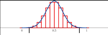
As Discussed above, when we increase the sample size, the sampling distribution turns into an approximate normal distribution.

For a sample distribution of a sample proportion, a rule of thumb is that the Central Limit Theorem is approximately observable in the distribution when np>=5 and n(1-p)>=5

For the Sampling Distribution of the Sample Proportion:

1. Center: The center of the sampling distribution is the population population
2. Spread: The width of the sampling distribution decreases as the number of people in our sample increases. The standard deviation of the distribution of samples is equal to \(\frac{\sqrt{p(1-p)}}{\sqrt{n}}\) and is called the standard error of the sample proportion
3. Shape: If n is large enough, we can appeal to the central limit theorem: the shape of the distribution of the sample proportion is approximately normal

---

Confidence Intervals

Using the Central Limit Theorem and the Standard error, We could work out the range of values that the parameter of interest lies

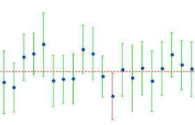
• A 95% confidence interval means that for 95% of the time, the value would lie within the given range of the confidence interval.
• As you shrink the interval towards the mean of the sampling distribution, the confidence would decrease.

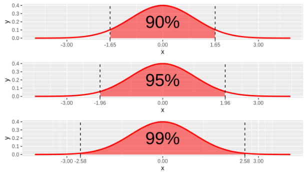
In other words, the probability of the statistic lying between these intervals would be the confidence interval. For example, if the confidence interval is 95%, and the range is [a,b], then p(a<x<b)=0.95.

Confidence interval for a proportion:

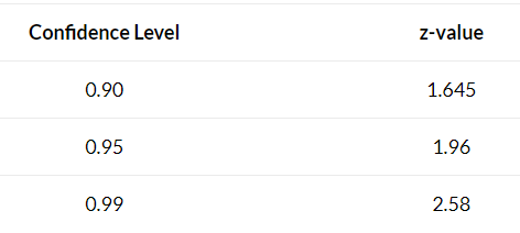
Confidence Interval = (point estimate)  +/-  (critical value)*(standard error)

Confidence Interval for sample mean= \(\bar{x}\pm z* (\frac{s}{\sqrt(n)})\)

Confidence Interval for sample proportion= \(\bar{p}\pm z* \sqrt(\frac{p(1-p)}{n})\) ,